
🔑 In 10 minutes you will learn:
- How GANs Work
Generative Adversarial Networks commonly known as GANs are computational architectures that set two neural networks against each other (thus the name “adversarial”), to create new examples of data that fulfill the characteristics of real data. While GANs have a lot of applications, they are typically used in image, video, or speech generation.
In 2014, Ian Goodfellow, Yoshua Bengio and several academics at the University of Montreal, published a paper that introduced GANs. Referring to the impressive capabilities of GANs, Yann LeCun, research director at Facebook AI dubbed adversarial training “the most fascinating notion in machine learning in the last 10 years”.
To develop and modify new data, Ian Goodfellow’s GANs suggest using two neural networks. One is the generator network responsible for creating new instances of data. To put it simply, the process is the inverse of the classification method of neural networks. Unlike the other neural networks, the generator doesn’t take the raw data and map it to predetermined model outputs. Instead it goes backwards from the output in an attempt to construct the input data that would then be mapped to that output. A generator network in GANs, for example, may start off with a matrix of pixels (consisting of random noise) and try to change them in such a manner that a classifier would categories them as a cat.
The second neural network in GANs is called the discriminator. On a scale of 0 to 1, it assesses the quality rating of the generator’s output. If the quality score is less than the desired level, the data is corrected by the generator and sent back to the discriminator. The GAN continues the loop in super-fast fashion until it reaches a point where it can generate data that accurately maps to the intended output.

Overview of GANs: Source
In the original paper of GANs titled “Generative Adversarial Networks” Ian Goodfellow, et al. used three datasets (namely MNIST, CIFAR-10, and Toronto Face Database) to generate new images. So, generating new sample examples was the main application of GANs described in the paper.
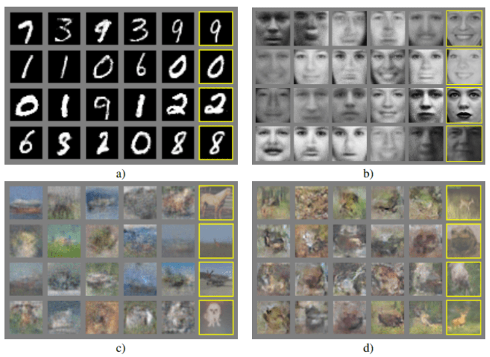
New Examples of Images Generated by GANs: Source
Likewise, in 2015 Alec Radford, et al. introduced Deep Convolutional Generative Adversarial Networks in his paper “Unsupervised Representation Learning with Deep Convolutional Generative Adversarial Networks”. He also generated new realistic images of bedrooms and presented his analysis on training stable GANs.
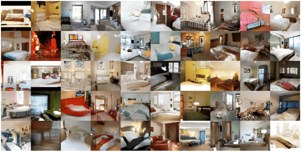
New Examples of Bedroom Images Generated by DCGANs: Source
Let’s not wait any longer and go into the implementation specifics of GANs as we go. Here we’ll demonstrate how we can use Deep Convolutional Generative Adversarial Network implementation (DCGAN) to generate realistic images. In our implementation, Tensorflow is used, and some of the principles stated in the DCGAN paper are followed.
We’ll train our DCGAN on Fashion-MNIST dataset comprising of 70,000 28×28 grayscale images with 60,000 images for training and 10,000 images for testing. Plus, it includes 10 classes of products.
So, before we start, let’s import some necessary packages we’ll use in this implementation.
import tensorflow as tf
import tensorflow.keras as keras
import matplotlib.pyplot as plt
import numpy as np
from IPython import display
We’ll use some helper functions to visualize the results in the later sessions.
def visualize_images(sample_images, columns=None):
    '''displaying fake examples'''
    display.clear_output(wait=False)

    columns = columns or len(sample_images)
    rows = (len(sample_images) - 1) // columns + 1

    if sample_images.shape[-1] == 1:
        sample_images = np.squeeze(sample_images, axis=-1)

    plt.figure(figsize=(columns, rows))

    for index, sample_image in enumerate(sample_images):
        plt.subplot(rows, columns, index + 1)
        plt.imshow(sample_image, cmap="binary")
        plt.axis("off")
After downloading the Fashion-MNIST dataset, training images are converted into batches. Then we’ll apply some basic preprocessing steps.
# downloading the Fashin-MNIST dataset
from keras.datasets import fashion_mnist
(X_train, _), _ = fashion_mnist.load_data()

# normalizing the images
X_train = X_train.astype(np.float32) / 255

# reshape and rescale
X_train = X_train.reshape(-1, 28, 28, 1) * 2. - 1.

#defining the batch size
batch_size = 64

# creating batches of tensors before feeding them into the model
data_set = tf.data.Dataset.from_tensor_slices(X_train)
data_set = data_set.shuffle(1000)
data_set = data_set.batch(batch_size, drop_remainder=True).prefetch(1)
The generator network takes random noise samples as inputs. They are eventually transformed into the shape of Fashion-MNIST images. Following the steps below, let’s build a generator network for a DCGAN.
- We’ll feed the noise samples as input to the dense layer of the network.
- The output of the network will be reshaped in order to form three dimensions. This goes for length, width, and number of filters.
- We’ll perform the deconvolution operation with Conv2DTranspose and set the stride at 2.
- The number of filers shall be reduced by half at each level of the network.
- We perform upsampling operation in order to match the feature size of the training images. In this case, it should be 28 x 28 x 1.
- Batch Normalization layer is added after every convolution layer except for the final deconvolution layer.
- As best practice, we use SELU (Scaled Exponential Linear Unit) activation function for intermediate deconvolution operations.
- Similarly for the output layer, tanh is used.
Let’s code everything described above in a block and print out the model summary in order to check the dimensions and shapes at each layer.
from keras.models import Sequential
from keras.layers import Dense, Reshape, BatchNormalization, Conv2DTranspose, Conv2D, Dropout, Flatten
codings_size = 32

def generator_nn(codings_size):
  generator = Sequential([Dense(7 * 7 * 128, input_shape=[codings_size]),
                          Reshape([7, 7, 128]),
                          BatchNormalization(),
                          Conv2DTranspose(64, kernel_size=5, strides=2, padding="SAME",
                                          activation="selu"),
                          BatchNormalization(),
                          Conv2DTranspose(1, kernel_size=5, strides=2, padding="SAME",
                                          activation="tanh"),
                          ])
  return generator

# get the generator network and print out the summary
gen = generator_nn(codings_size)
gen.summary()
Model: "sequential"
_________________________________________________________________
 Layer (type)                Output Shape              Param #
=================================================================
 dense (Dense)               (None, 6272)              206976

 reshape (Reshape)           (None, 7, 7, 128)         0

 batch_normalization (BatchN  (None, 7, 7, 128)        512
 ormalization)

 conv2d_transpose (Conv2DTra  (None, 14, 14, 64)       204864
 nspose)

 batch_normalization_1 (Batc  (None, 14, 14, 64)       256
 hNormalization)

 conv2d_transpose_1 (Conv2DT  (None, 28, 28, 1)        1601
 ranspose)

=================================================================
Total params: 414,209
Trainable params: 413,825
Non-trainable params: 384
_________________________________________________________________
Similarly, we’ll build a discriminator network using the following steps:
- Use the convolutional layers by setting the strides at 2 in order to reduce the size or dimensions of the input images.
- Use “LeakyRELU” as an activation function after every convolution operation.
- Flatten the output features and feed them to a dense layer with single neuron activated by “sigmoid” activation function.
The implementation details along with the model summary are as under.
# building the discriminator network

def discriminator_nn():
  discriminator = Sequential([
                              Conv2D(64, kernel_size=5, strides=2, padding="SAME",
                                     activation=keras.layers.LeakyReLU(0.2),
                                     input_shape=[28, 28, 1]),
                              Dropout(0.3),
                              Conv2D(128, kernel_size=5, strides=2, padding="SAME",
                                     activation=keras.layers.LeakyReLU(0.2)),
                              Dropout(0.4),
                              Flatten(),
                              Dense(1, activation="sigmoid")
])
  return discriminator
discrim = discriminator_nn()
discrim.summary()
Model: "sequential_11"
_________________________________________________________________
 Layer (type)                Output Shape              Param #
=================================================================
 conv2d_6 (Conv2D)           (None, 14, 14, 64)        1664

 dropout_6 (Dropout)         (None, 14, 14, 64)        0

 conv2d_7 (Conv2D)           (None, 7, 7, 128)         204928

 dropout_7 (Dropout)         (None, 7, 7, 128)         0

 flatten_2 (Flatten)         (None, 6272)              0

 dense_9 (Dense)             (None, 1)                 6273

=================================================================
Total params: 212,865
Trainable params: 212,865
Non-trainable params: 0
_________________________________________________________________
Now, let’s combine these two neural networks (i.e. generator and discriminator) for a complete architecture of a DCGAN. Here is how we’ll do that.
#combining the generator and discriminator
dcgan = Sequential([gen, discrim])
As the model distinguishes between fake (0) and real (1), we’ll use “binary_crossentropy” in order to measure the loss between the images. Moreover, we’ll optimize the model loss with RMS_prop optimizer. Let’s now compile the model for training.
# compiling the model
discrim.compile(loss="binary_crossentropy", optimizer="rmsprop")
discrim.trainable = False
dcgan.compile(loss="binary_crossentropy", optimizer="rmsprop")
Let’s define a function that trains our GAN on a given batch of images. The process involves two-phase training steps as under:
- First off, we’ll train our discriminator network in order to distinguish between real and fake images.
- Next, the generator network will be trained to produce fake images that should trick the discriminator to map them as real ones.
def train_dcgan(dcgan, data_set, random_normal_dimensions, epochs=20):
    gen, discrim = dcgan.layers
    for epoch in range(epochs):
        print("Epoch {}/{}".format(epoch + 1, epochs))
        for real_image_samples in data_set:
            # infer batch size from the training batch
            batch_size = real_image_samples.shape[0]

            # Training the discriminator network - first phase
            # creating random noise samples
            noise_samples = tf.random.normal(shape=[batch_size, random_normal_dimensions])

            # generating fake image samples
            fake_image_samples = gen(noise_samples)

            # listing fake and real images by concatinating them
            conc_images = tf.concat([fake_image_samples, real_image_samples], axis=0)

            # Create the labels for the discriminator
            # 0 for the fake images
            # 1 for the real images
            discrim_labels = tf.constant([[0.]] * batch_size + [[1.]] * batch_size)

            # set the discriminator to trainable
            discrim.trainable = True

            # training the discriminator on the batches of conc_images and the discrim_labels
            discrim.train_on_batch(conc_images, discrim_labels)

            # Training the generator netwrok - 2nd phase
            # feeding noise input samples into DCGAN
            noise_samples = tf.random.normal(shape=[batch_size, random_normal_dimensions])

            # labelling generated images as real images
            gen_labels = tf.constant([[1.]] * batch_size)

            # freezing the discriminator network
            discrim.trainable = False

            # training the DCGAN with labels set to true
    dcgan.train_on_batch(noise_samples, gen_labels)

# plotting fake image samples
visualize_images(fake_image_samples, 16)
plt.show()
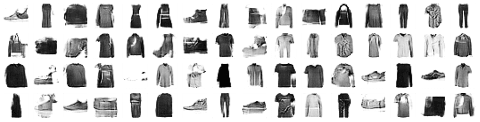
Finally, it’s time to train our DCGAN and see the magic. We’ll call the above function to start the training. While we set the number of epochs to 20, you are free to try the higher number in order to achieve more accuracy. It should take around 30 seconds to execute single epoch in a colab environment. You will visualize the results (fake images generated by our DCGAN) after every epoch during the training process.
So, let’s start off the training by simply executing the below lines of code.
#trining the DCGAN for 20 epochs
train_dcgan(dcgan, data_set, codings_size, 20)
After the training, your final output should look like this.
In machine learning community, GANs have been one of the hottest topics due to their impressive capabilities. These models can take the unsupervised learning methods to new heights, hence broadening the scope of machine learning.
Since its inception, many strategies for training GANs have been developed by the researchers. They have been able to introduce some new and state-of-the-art training strategies that can be employed in image/video generation and semi-supervised learning.