Image preprocessing and augmentation are important steps before you train statistical algorithms e.g machine learning models on images. Image preprocessing and augmentation can help increase dataset size by generating similar copies of images. It can also improve data versatility which helps improve model generalisation and reduces overfitting.
In this article, you will see how to preprocess and augment input images using TensorFlow keras library. The article also demonstrates how image preprocessing can help improve a deep learning model performance in TensorFlow keras.
Downloading Sample Dataset
The sample dataset for this article can be downloaded from this Kaggle Link:
https://www.kaggle.com/datasets/cmranzd/dogs-vs-cats-small-data
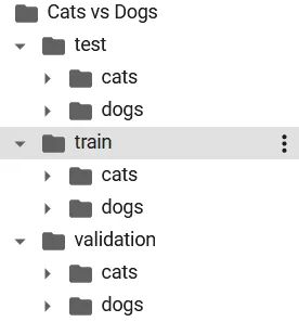
The dataset consists of images of cats and dogs. Once you download the dataset, you will see that it contains three folders: test, train, and validation. Each of these three folders further consist of two sub-folders: cats and dogs, which contain unique images of cats, and dogs, respectively.
The directory structure for your dataset looks like this:
Preprocessing and Augmenting Images
In this section, you will see how to preprocess and apply augmentation to in-memory images using TensorFlow keras.
To preprocess and augment images with TensorFlow keras, you can use the Image submodule from the https://www.tensorflow.org/api_docs/python/tf/keras/preprocessing/image/ module. The ImageDataGenerator class from the image module preprocesses and augments images on the fly as you will see in the upcoming sections.
The following script imports this module along with the other libraries required to run codes in this section.
import numpy as np

import matplotlib.pyplot as plt

from keras.preprocessing import image
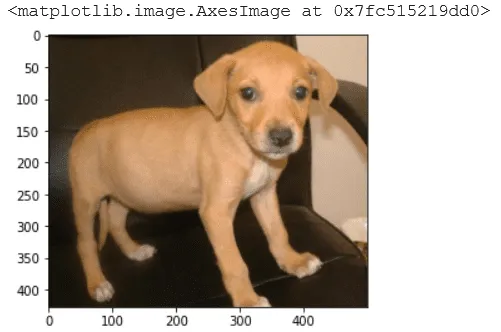
The script below imports an image of a dog from the train dataset. The image is then displayed using the “imshow()” method.
#load the image
img = image.load_img('/content/Cats vs Dogs/train/dogs/dog.117.jpg')

plt.imshow(img)
Output:
To apply preprocessing via the Keras.preprocessing.image module, you need to convert an input image into a numpy array. You can do so using the “img_to_array()” method as shown below:
#convert to numpy array
img_array = image.img_to_array(img)

print(img_array.shape)
Output:
(427, 500, 3)
The script above plots the image shape. You can see the height, width, and the colour channels from the above output.
Most of the keras.preprocessing.image module functionalities including the ImageDataGenerator, expect the images in the format (number of samples, height, width, number of colour channels). In our case, we have only one image and hence one sample. The following script adds the number of samples dimension to the input image.
from numpy import expand_dims

img_arrays = expand_dims(img_array, 0)

print(img_arrays.shape)
Output:
(1, 427, 500, 3)
Let’s now see some of the most common preprocessing and image augmentation features of the ImageDataGenerator class.
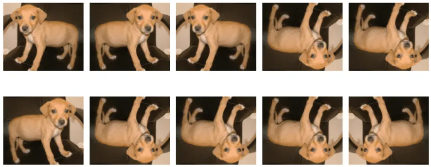
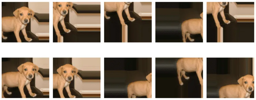
Horizontal and Vertical Flips
To horizontally and/or vertically flip input images, you need to set the horizontal_flip, and vertical_flip attributes of the ImageDataGenerator class to True.
img_data_gen = image.ImageDataGenerator(horizontal_flip=True, vertical_flip= True)
Next, to actually generate preprocessed images using in memory images as inputs, you need to call the “flow()” method using the ImageDataGenerator class object. The input image array and the value for the batch_size attribute is passed as attributes to the “flow” method. Since we have only a single image, we set the batch size to 1.
data_gen_iterator = img_data_gen.flow(img_arrays, batch_size = 1)
In the script below, the “flow()” method is called 10 times, and every time the original or flipped version of the input image is generated, which is then displayed.
plt.figure(figsize=(10,6))

for i in range(10):

plt.subplot(2,5,i+1)

batch = data_gen_iterator.next()

plt.imshow(batch[0].astype('uint8'))

plt.axis('off')

plt.tight_layout()

plt.show()
Output:
Height and Width Shifts
You can shift an image certain number of pixels horizontally or vertically using the
Width_shift_range, and height_shift_range attributes respectively. Setting a float value between 0-1 applies a relative shift. For instance a value of 0.5 shifts 50% of an image whereas a value greater than 1 is treated as the number of pixels.
Here is an example:
img_data_gen = image.ImageDataGenerator(width_shift_range=0.5, height_shift_range= 200)

data_gen_iterator = img_data_gen.flow(img_arrays, batch_size = 1)

plt.figure(figsize=(10,5))

for i in range(10):

plt.subplot(2,5,i+1)

batch = data_gen_iterator.next()

plt.imshow(batch[0].astype('uint8'))

plt.axis('off')

plt.tight_layout()

plt.show()
Output:
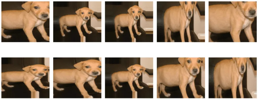
Rotating Images
You can rotate images by passing angle value in degrees to the rotation_range attribute of the ImageDataGenerator class. The following script rotates images by upto -90 to 90 degrees.
img_data_gen = image.ImageDataGenerator(rotation_range = 90)

data_gen_iterator = img_data_gen.flow(img_arrays, batch_size = 1)

plt.figure(figsize=(10,5))

for i in range(10):

plt.subplot(2,5,i+1)

batch = data_gen_iterator.next()

plt.imshow(batch[0].astype('uint8'))

plt.axis('off')

plt.tight_layout()

plt.show()
Output:
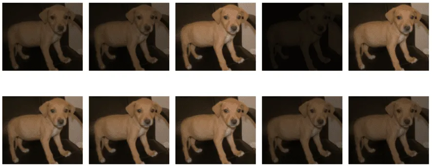
Adjusting Image Brightness
You can also adjust image brightness. To do so you need to pass a tuple of values specifying relative minimum and maximum brightness, to the brightness_range attribute. For instance, a brightness value of (0.1, 1) will generate images with brightness levels of 10% to
img_data_gen = image.ImageDataGenerator(brightness_range = (0.1,1))

data_gen_iterator = img_data_gen.flow(img_arrays, batch_size = 1)

plt.figure(figsize=(10,5))

for i in range(10):

plt.subplot(2,5,i+1)

batch = data_gen_iterator.next()

plt.imshow(batch[0].astype('uint8'))

plt.axis('off')

plt.tight_layout()

plt.show()
Output:
Zooming Images
To apply zoom on images, you have to pass a tuple to the zoom_range attribute. The tuple specifies relative minimum and maximum zoom values, respectively. Here is an example:
img_data_gen = image.ImageDataGenerator(zoom_range = (0.5,1.5))

data_gen_iterator = img_data_gen.flow(img_arrays, batch_size = 1)

plt.figure(figsize=(10,5))

for i in range(10):

plt.subplot(2,5,i+1)

batch = data_gen_iterator.next()

plt.imshow(batch[0].astype('uint8'))

plt.axis('off')

plt.tight_layout()

plt.show()
Output:
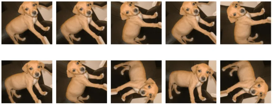
Applying Shear
You can also apply shear to images to make them appear stretched. The angle of shear needs to be passed to the shear_range attribute.
img_data_gen = image.ImageDataGenerator(shear_range = 45)

data_gen_iterator = img_data_gen.flow(img_arrays, batch_size = 1)

plt.figure(figsize=(10,5))

for i in range(10):

plt.subplot(2,5,i+1)

batch = data_gen_iterator.next()

plt.imshow(batch[0].astype('uint8'))

plt.axis('off')

plt.tight_layout()

plt.show()
Output:
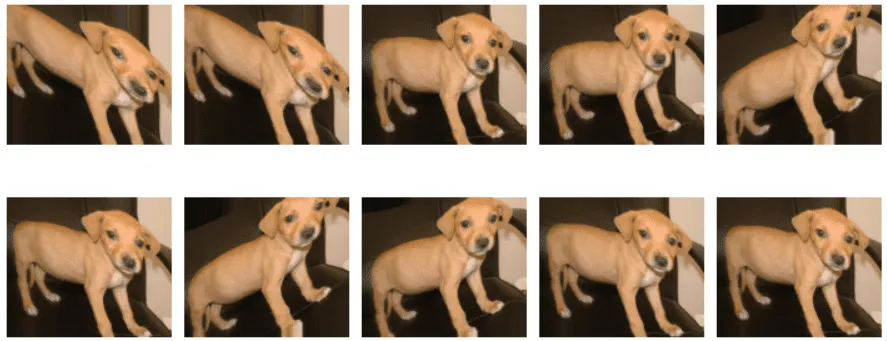
Image Classification without Image Preprocessing and Augmentation
In this section, you will train a convolutional neural network for the classification of cats and dog images in your dataset. We will be using the default images without any preprocessing and augmentation to see what is the maximum prediction accuracy that our model can achieve when we do not apply any preprocessing or augmentation to our images.
In the previous section you saw how to preprocess and augment images that reside in the computer’s memory in the form of numpy arrays.
In the case of huge datasets, it is not convenient to keep all your images in the computer’s memory. Rather, the images are stored in directories on the system’s harddrive. The images are then retrieved in batches and subsequent operations are performed on it.
The process of preprocessing images residing in directories is similar to preprocessing in-memory images that you saw in the previous section. However the process of loading images will be different, which you will see in this section.
The following script defines variables that store the paths to train, test and validation folders in our dataset.
train_images = '/content/Cats vs Dogs/train'

test_images = '/content/Cats vs Dogs/test'

val_images = '/content/Cats vs Dogs/validation'
The script below displays the total number of images in train, test and validation folders.
training_files = glob(train_images + '//.jp*g')

test_files = glob(test_images + '//.jp*g')

val_files = glob(val_images + '//.jp*g')

print("Number of training images: ",len(training_files))

print("Number of test images: ",len(test_files))

print("Number of val images: ",len(val_files))
Output:
Number of training images: 2000
Number of test images: 1000
Number of val images: 1000
The following script creates ImageDataGenerator objects for the images in train, test, and validation folders. The only preprocessing step applied is dividing the pixel values by 255 in order to normalise the dataset.
train_gen = image.ImageDataGenerator(rescale = 1./255)

test_gen = image.ImageDataGenerator(rescale = 1./255)

val_gen = image.ImageDataGenerator(rescale = 1./255)
In the previous section you used the “flow()” method to create an iterator that returns images. To create an iterator that loads images from directories, you need to call the “flow_from_directory()” method as shown in the script below.
You need to pass the path to the directory and the batch size as parameter values. The iterator in the script below, resizes the input images into 400 x 400 pixel images. A batch size of 16 images is processed at a time for training. And finally, the “class_mode” attribute is set to “binary” since there are only two output classes in our dataset.
training_data_iter = train_gen.flow_from_directory(train_images,

target_size = (400, 400),

batch_size = 16,

class_mode = 'binary')

test_data_iter = test_gen .flow_from_directory(test_images,

target_size = (400, 400),

batch_size = 16,

class_mode = 'binary')

val_data_iter = val_gen.flow_from_directory(val_images,

target_size = (400, 400),

batch_size = 16,

class_mode = 'binary')
Output:
Found 2000 images belonging to 2 classes.
Found 1000 images belonging to 2 classes.
Found 1000 images belonging to 2 classes.
Finally, the script below defines our convolutional neural network model for classification. The model consists of an input layer, three convolutional and subsequent maxpool layers, followed by a dense layer and an output layer.
import numpy as np

import matplotlib.pyplot as plt

from keras.layers import Input, Conv2D, Dense, Flatten, Dropout, MaxPool2D

from keras.models import Model

input = Input(shape = (400, 400, 3) )

convol1 = Conv2D(64, (3,3), strides = 2, activation= 'relu')(input)

maxpool1 = MaxPool2D(2, 2)(convol1)

convol2 = Conv2D(32, (3,3), strides = 2, activation= 'relu')(maxpool1)

maxpool2 = MaxPool2D(2, 2)(convol2)

convol3 = Conv2D(16, (3,3), strides = 2, activation= 'relu')(maxpool2)

maxpool3 = MaxPool2D(pool_size = (2, 2))(convol3)

flat_layer1 = Flatten()(maxpool3)

dense_layer1 = Dense(256, activation = 'relu')(flat_layer1)

output = Dense(1, activation= 'sigmoid')(dense_layer1)

model = Model(input, output)
The following script compiles the model:
model.compile(optimizer = 'adam', loss= 'binary_crossentropy', metrics =['accuracy'])
And the script below trains our model on the images from the training set, while the trained model is validated on the validation.
steps_per_epo = len(training_files)/16

val_steps = len(test_files)/16

model_hist = model.fit(training_data_iter,

steps_per_epoch = steps_per_epo ,

epochs=20,

validation_data = val_data_iter,

validation_steps = val_steps,

verbose=1)
The output below shows that after 20 epochs, the model achieves an accuracy of 65.80% on the validation set.
Output:
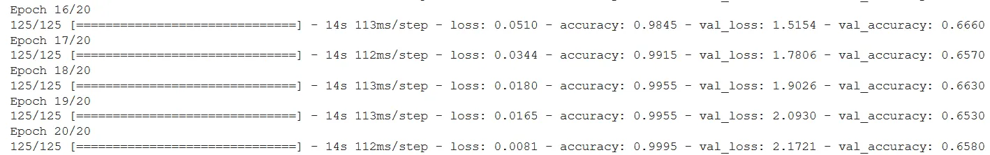
The following script plots the training and validation accuracies:
import matplotlib.pyplot as plt

plt.figure(figsize=(10,6))

plt.plot(model_hist.history['accuracy'], label = 'accuracy')

plt.plot(model_hist.history['val_accuracy'], label = 'validation_accuracy')

plt.legend(['train','validation'], loc='lower left')
The plot below shows that the training accuracy reaches upto 95% while the validation accuracy is around 65%. This shows that our model is clearly overfitting.
Output:
Finally, let’s make predictions on the unseen test set.
test_scores  = model.evaluate(test_data_iter, verbose=0)

print('Test loss:', test_scores[0])

print('Test accuracy:', test_scores[1])
The output below shows that we get an accuracy of 66.90 % on the unseen test set.
Output:
Test loss: 2.0298449993133545
Test accuracy: 0.6690000295639038
Image Classification without Image Preprocessing and Augmentation
Now let’s perform classification on cats and dog images again. However, this time you will be applying preprocessing and data augmentation on the training images.
It is important to mention that you should only apply image preprocessing and augmentation on your training data. As discussed earlier, preprocessing and augmenting images has two main advantages for machine learning algorithms:
- It can help increase the dataset size by generating similar copies of existing images.
- It increases versatility of images in a dataset which helps reduce overfitting for classification tasks.
Let’s see how image preprocessing and augmentation will help improve model performance and remove overfitting.
The script below creates an ImageDataGenerator object that applies horizontal flip, rotation, zooming, and shear preprocessing steps to the training images. Notice, we did not apply any preprocessing to the test and validation images.
train_gen = image.ImageDataGenerator(rescale = 1./255,

horizontal_flip= True,

rotation_range= 30,

zoom_range = (0.8,1.2),

shear_range = 0.2

)

test_gen = image.ImageDataGenerator(rescale = 1./255)

val_gen = image.ImageDataGenerator(rescale = 1./255)
The rest of the process is similar to what you have seen in the previous section. The script below creates image iterators for train, test, and validation sets.
training_data_iter = train_gen.flow_from_directory(train_images,

target_size = (400, 400),

batch_size = 16,

class_mode = 'binary')

test_data_iter = test_gen .flow_from_directory(test_images,

target_size = (400, 400),

batch_size = 16,

class_mode = 'binary')

val_data_iter = val_gen.flow_from_directory(val_images,

target_size = (400, 400),

batch_size = 16,

class_mode = 'binary')
Output:
Found 2000 images belonging to 2 classes.
Found 1000 images belonging to 2 classes.
Found 1000 images belonging to 2 classes.
The script below defines your convolutional neural network model.
import numpy as np

import matplotlib.pyplot as plt

from keras.layers import Input, Conv2D, Dense, Flatten, Dropout, MaxPool2D

from keras.models import Model

input = Input(shape = (400, 400, 3) )

convol1 = Conv2D(64, (3,3), strides = 2, activation= 'relu')(input)

maxpool1 = MaxPool2D(2, 2)(convol1)

convol2 = Conv2D(32, (3,3), strides = 2, activation= 'relu')(maxpool1)

maxpool2 = MaxPool2D(2, 2)(convol2)

convol3 = Conv2D(16, (3,3), strides = 2, activation= 'relu')(maxpool2)

maxpool3 = MaxPool2D(pool_size = (2, 2))(convol3)

flat_layer1 = Flatten()(maxpool3)

dense_layer1 = Dense(256, activation = 'relu')(flat_layer1)

output = Dense(1, activation= 'sigmoid')(dense_layer1)

model = Model(input, output)
The following script compiles the model:
model.compile(optimizer = 'adam', loss= 'binary_crossentropy', metrics =['accuracy'])
Finally, the script below trains the model:
steps_per_epo = len(training_files)/16

val_steps = len(test_files)/16

model_hist = model.fit(training_data_iter,

steps_per_epoch = steps_per_epo ,

epochs=20,

validation_data = val_data_iter,

validation_steps = val_steps,

verbose=1)
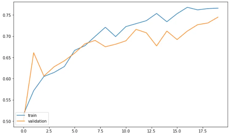
The output shows that at the end of 20 epochs, our model achieves the validation accuracy of 74.50% which is much better than 65.80% which was achieved by the model trained on non-preprocessed images.
Output:
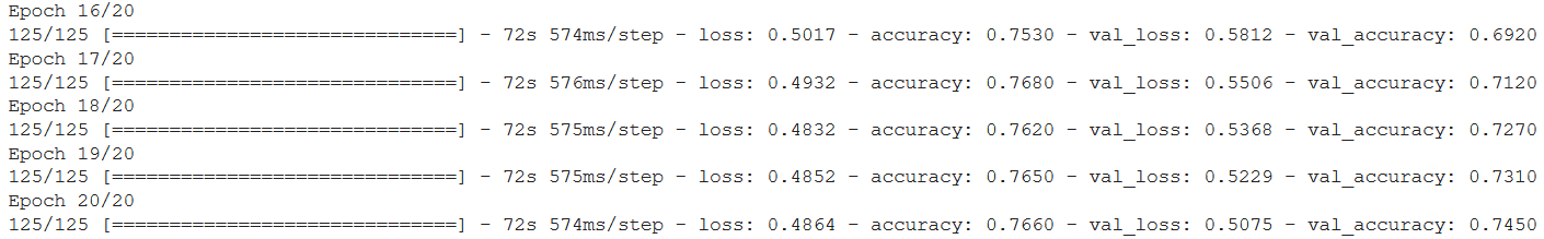
The output below shows that the overfitting in this case is much lower compared to the previous model. At the end of 20 epochs, the training accuracy is 76.60 while the validation accuracy is 74.50%.
Output:
The following script evaluates the model performance on the test set.
test_scores  = model.evaluate(test_data_iter, verbose=0)

print('Test loss:', test_scores[0])

print('Test accuracy:', test_scores[1])
Output:
Test loss: 0.5988056659698486
Test accuracy: 0.7139999866485596
The output above shows that a model returns an accuracy of 71.39% on the test set which is better than 66.90% achieved via model trained on images that are not preprocessed.
Image preprocessing and augmentation is an important preprocessing step for training deep learning algorithms. This article demonstrates how to use different preprocessing and data augmentation techniques available in the TensorFlow Keras preprocessing.image module.
The results show that preprocessing and augmenting images can help improve a deep learning model’s accuracy. The choice of preprocessing techniques, however, depend upon the domain knowledge. For instance, in some cases you might need to flip images horizontally while in other cases it wont make any difference on image appearance.