
Missing data, as the name suggests, are data observations that do not contain any value. Missing values can have a huge impact on the performance of data science models. Therefore, it is important to understand the reasons behind missing data, and the techniques that can be adopted to handle missing data.
In this article, you will study some of the common reasons for having missing data in your observations. Finally, you will study how to handle missing values in data stored in Pandas dataframe, which is one of the most common structures for storing data in the Python programming language.
Reasons for Missing Data
There can be multiple reasons for having missing data in your observations. Three of the most common reasons are listed below:
- Sometimes the data is not recorded intentionally. For instance, while completing market surveys, some people might not enter their annual revenue. In such cases, you will have missing observations in your data.
- The data is oftentimes not available at the time when the observation is recorded. For instance, some of the information about the patients who are brought to emergencies in hospitals might not be immediately available at the time of registering patients.
- Information is often lost due to technical reasons or calculations. For instance, you might have recorded a person’s weight in a computer but due to application crashing or power failure the data is not recorded.
Types of Missing Data
Missing data can be divided into three main categories:
Missing Data Completely Randomly
If a missing observation for a particular attribute doesn’t have any relation with other attributes, we can say that the data is missing completely randomly. For instance, if a person forgets to write his city name in a survey, you can say that this data is missing completely randomly since there is no other logical conclusion of missing data.
Missing Data Randomly
In case if a missing observation has a relationship with one of the other attributes of the data, we can say that the data is missing randomly. For instance, it is likely that overweight patients do not write their weights while filling marketing surveys, in such cases we can say that the data is missing randomly
Missing Data Not Randomly
Disadvantages of Missing Data
There are multiple disadvantages of having missing data in your datasets. Some of the disadvantages are enlisted below:
- Some data science and machine learning tools such as Scikit learn don’t expect your data to have missing values. You have to either remove or somehow handle missing values before you could feed your data to train models from these libraries,
- The data imputation techniques may distort the overall distribution of your data.
Enough of the theory, let’s now see some of the techniques used for handling missing data stored in Pandas dataframes in Python.
Importing and Analysing the Dataset for Missing Values
The dataset that you will be using in this article can be downloaded in the form of a CSV file from the following Kaggle link.
https://www.kaggle.com/code/dansbecker/handling-missing-values/data?select=melb_data.csv
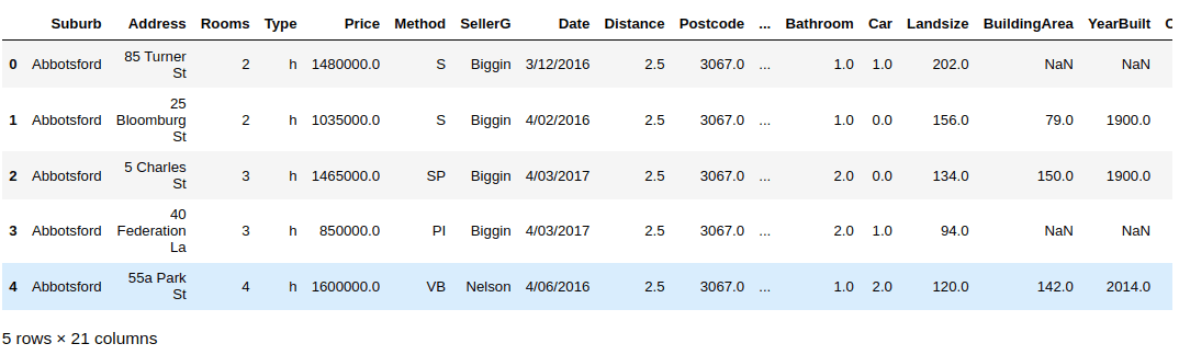
The script below imports the dataset and displays its header.
import pandas as pddata_path = "/home/manimalik/Datasets/"house_data = pd.read_csv(data_path + "melb_data.csv")house_data.head()
The database consists of information about houses in Melbourn (city of Australia). Some of the data attributes are Room, Price, Postcode, Building Area, Year Built etc.
Output:
Let’s try to see the number of records in our dataset.
house_data.shape
Output:
(13580, 21)
The dataset consists of 13580 records and 21 attributes.
Next, let’s try to see which attributes or columns contain null values.
house_data.isnull().sum()
Output:
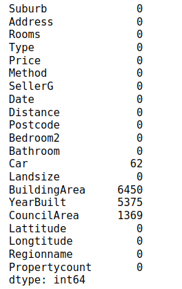
From the above output, you can see that Car, BuildingArea, YearBuilt, and CouncilArea are the columns having missing data. The BuildingArea attribute has null values in 6450 records which is almost 47.50% of the total dataset.
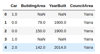
Let’s filter the columns with the missing values. We will be working with these columns only for handling missing data.
house_data = house_data.filter(["Car", "BuildingArea", "YearBuilt", "CouncilArea"])house_data.head()
Output:
Finally, let’s try to print the data types of the columns having missing values.
house_data.dtypes
Output:
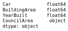
The above output shows that Car, BuildingArea, and YearBuilt are numeric attributes (of type float), whereas only the CouncilArea attribute contains categorical values.
Remove Complete Rows or Columns with Missing Data
The first and the simplest approach of handling missing data is by removing all the records where any column contains missing value. Or alternatively, you can also drop a column if the majority of values in that column is null.
Let’s try to remove all the rows containing null values from our sample dataset.
house_data_filteres = house_data.dropna()print(house_data_filteres.shape)
Output:
(6196, 21)
After removing all the rows where any column contains a null or missing value, we are left with only 6196 records.
Another option is to only remove those rows where a specific column contains missing values. For example, the script below removes all the rows where the BuildingArea attribute contains null values.
house_data_filteres = house_data[house_data['BuildingArea'].notna()]print(house_data_filteres.shape)
Output:
(7130, 21)
The main advantage of removing all the rows containing missing values is that this technique is extremely simple to implement and works for both numeric and categorical data types.
The main disadvantage of removing rows with missing values is that if a large number or rows contain missing values, you will lose a large chunk of useful data contained in attributes that do not have any missing values.
As a rule of thumb, handle missing data by removing rows only if less than 5% of the rows contain missing data.
In addition to removing complete rows, imputation techniques exist that can be used to fill missing data by inferencing values via interpolation from the dataset. In the next sections, you will see imputation techniques for handling missing numeric and categorical data.
Handling Numeric Missing Values using Imputation
The main imputation techniques for handling missing numeric values are:
- Mean/Median Imputation
- End of Distribution Imputation
- Arbitrary Value Imputation
Mean Median Imputation
In mean or median imputation, as the name suggests, the numerical missing data for an attribute is replaced by the mean or median of the remaining values for that attribute.
As an example, we will perform mean or median imputation for missing values in the BuildingArea attribute of our dataset.
The script below calculates the median and mean values for the BuildingArea attribute.
median_BuildingArea = house_data.BuildingArea.median()print("Median of BuildingArea:", median_BuildingArea)mean_BuildingArea = house_data.BuildingArea.mean()print("Mean of BuildingArea:", mean_BuildingArea) The main imputation techniques for handling missing numeric values are:
- Mean/Median Imputation
- End of Distribution Imputation
- Arbitrary Value Imputation
Output:
Median of BuildingArea: 126.0
Mean of BuildingArea: 151.96764988779805
As a next step, we will create two new columns in our dataset:
- Median_BuildingArea: that will contain the median value of the BuidingArea attribute for the rows that contain a missing or null value in the BuildingArea column.
- Mean_BuildingArea: column will contain the mean value of the BuidingArea attribute for the rows that contain a missing or null value in the BuildingArea column.
The following script performs the mean and median imputation for the BuildingArea attribute.
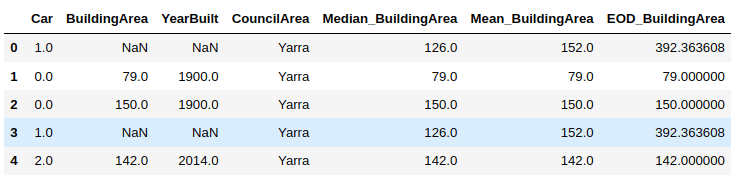
import numpy as nphouse_data['Median_BuildingArea'] = house_data.BuildingArea.fillna(median_BuildingArea)house_data['Mean_BuildingArea'] = np.round(house_data.BuildingArea.fillna(mean_BuildingArea), 1)house_data.head()
Output:
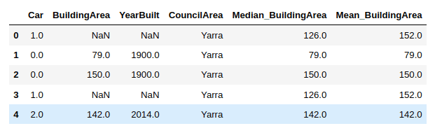
From the above output, you can see that the 1st and 4th rows contain a NaN (or null) value in the BuildingArea column. You can see the median and mean values for these rows in the Median_BuildingArea and Mean_BuildingArea columns, respectively.
The main advantage of the mean and median imputation is that they are extremely easy to calculate. Furthermore, the mean and median imputations can also be implemented during production. Mean and Median imputations are also good for data missing randomly.
The major disadvantage of the mean and median imputation is that they affect the default data distribution, particularly the variance of the data.
End of Distribution Imputation
For the data not missing randomly, the mean and median imputations are not good approaches. Rather the end of distribution imputation (also known as the end of tail imputation) is the commonly used technique. The end of distribution imputation tells the data model that the data is not missing randomly and hence cannot be inferred from the existing data via interpolation.
It is always a good practice to remove data outliers before performing the end of distribution imputation.
To view data outliers, you can plot a box plot.
import seaborn as snssns.boxplot(y=house_data['BuildingArea'])
Output:
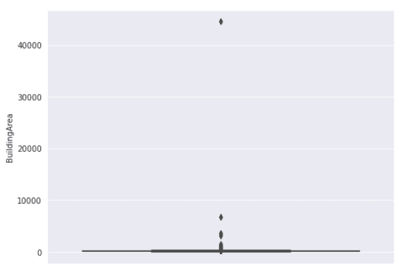
The box pot shows that most of our values are below 1000. The dots shown in the above figure are outliers.
Normally outliers are removed using interquartile range technique. However, for the sake of simplicity, we will simply remove the n-largest numbers from our dataset.
Let’s print the 10 largest values from the BuildingArea column.
house_data['BuildingArea'].nlargest(n=10)
Output:
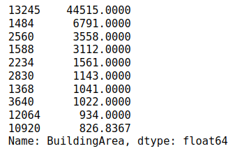
The output shows that the largest value is 44515 after that there is a huge difference of values and the second largest is 6791.
We remove all the values greater than 1000 from our dataset. As a result, 8 values will be removed.
house_data['BuildingArea'] = np.where(house_data['BuildingArea'] < 1000, house_data['BuildingArea'], np.nan)
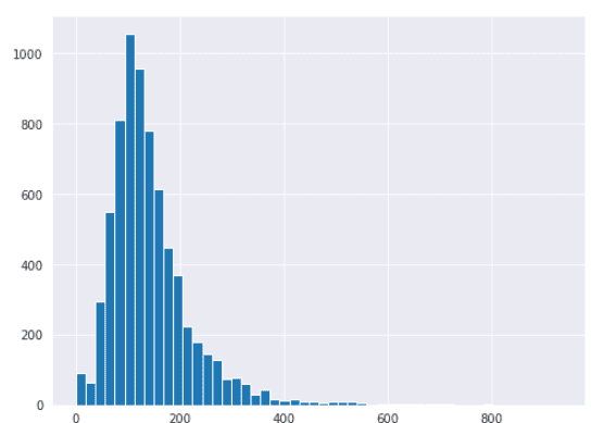
Now if you plot a histogram of values in the BuildingArea column, you will see that the data is normally distributed.
house_data['BuildingArea'].hist(bins=50)
Output:
Now you can perform the end of distribution. To do so, you have to multiply the mean value of the BuildingArea column with three standard deviations.
The script below finds the end of distribution value for the BuildingArea column.
end_of_val = house_data['BuildingArea'].mean() + 3 * house_data['BuildingArea'].std()print(end_of_val)
Output:
Arbitrary Value Imputation
In arbitrary value imputation, a totally arbitrary value is selected to replace missing values. The arbitrary value should not belong to the dataset. Rather, it signifies a missing value. A good value can be 99, 999, 9999 or any number containing the digit 9. In case of all positive values, you can use -1 as the arbitrary value.
In our dataset, the BuildingArea column only contains positive values. Therefore, to perform arbitrary value imputation, we create a new column i.e. AVE_BuildingArea that contains -1 for the rows where the original BuildingArea column contained missing data.
The following script performs the arbitrary value imputation for the BuildingArea column.
import numpy as nphouse_data['AVE_BuildingArea'] = house_data.BuildingArea.fillna(-1)house_data.head()
Output:
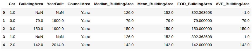
Arbitrary value imputation is also suitable for replacing data that is not missing randomly.
Handling Categorical Missing Values
Two main techniques exists for handling categorical missing values:
- Frequent Category Imputation
- Missing Category Imputation
Frequent Category Imputation
In arbitrary value imputation, a totally arbitrary value is selected to replace missing values. The arbitrary value should not belong to the dataset. Rather, it signifies a missing value. A good value can be 99, 999, 9999 or any number containing the digit 9. In case of all positive values, you can use -1 as the arbitrary value.
In our dataset, the BuildingArea column only contains positive values. Therefore, to perform arbitrary value imputation, we create a new column i.e. AVE_BuildingArea that contains -1 for the rows where the original BuildingArea column contained missing data.
The following script performs the arbitrary value imputation for the BuildingArea column.
import numpy as nphouse_data['AVE_BuildingArea'] = house_data.BuildingArea.fillna(-1)house_data.head()
The output below shows that “Moreland” council area is the most frequently occurring value in the CouncilArea column.
Output:
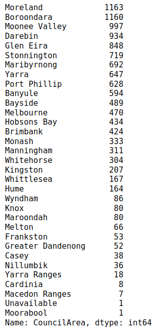
Another way to get the most frequently occurring value from a categorical column is by using the “mode()” method, as shown in the following script.
house_data['CouncilArea'].mode()

Output:

0    Moreland

dtype: object
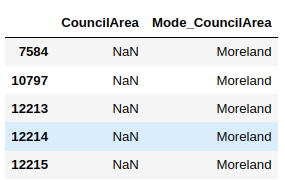
Now we know that the value “Moreland” is the most frequently occuring value in the CouncilArea column. We can replace the missing value in the CouncilArea column with this value and add them in a new column.
The following script does that and then prints the first five null values in the CouncilArea column along with the replaced values in the Mode_CouncilArea column.
house_data['CouncilArea'].mode() Output: 0 Moreland dtype: object
Output:
Frequent category imputation should be used when a categorical column contains randomly missing data.
Missing Category Imputation
In missing category imputation, missing values in a categorical column are simply replaced by any dummy value that does not exist in that column. Missing category imputation is used to tell the data models that the data is not missing at random and should not be replaced by any other value.
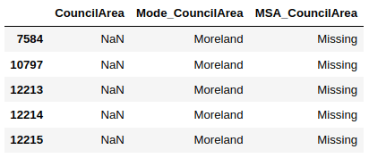
The following script creates a new column “MSA_CouncilArea” where the missing values from the CouncilArea column are replaced by the string “Missing”.
import numpy as nphouse_data['MSA_CouncilArea'] = house_data.CouncilArea.fillna("Missing") The script below shows the header of the original CouncilArea column containing null values, along with the “Mode_CouncilArea” column that displays the frequent category imputation values, and the “MSA_CouncilArea” column that contains the missing category imputation values.
house_data[house_data['CouncilArea'].isna()].filter(["CouncilArea", "Mode_CouncilArea", "MSA_CouncilArea"], axis = 1).head()
Output:
Missing values can hugely affect the performance of your data models. Therefore, it is immensely important to handle missing values in your datasets. To this end, several approaches exist for missing data handling as you saw in this article. However the decision to select a missing data handling technique depends on the type and the reason behind missing data.
As a rule of thumb, if less than 5% of records in your dataset contain missing values, you can simply remove those records. Else, if your numeric attribute contains missing data, and the data is missing randomly, you can select mean/median imputation. On the other hand if your numeric data is not missing randly, you should perform end of distribution, or arbitrary value imputation.
In case of categorical columns, if your data is randomly missing, frequent category imputation is the approach to go by. On the other hand if your categorical data are not missing randomly, you should opt for missing category imputation.