Image recognition can be divided into two processes; image detection and classification. Image detection is the first process where a set of algorithms are used to pre-process the image. Image classification then follows, here the image is put into its class. There has been a great improvement in the ability of computers to detect and classify images in the recent past. In this blog post, we are going to discuss some of the machine learning algorithms that are used for image classification. We are going to look at what they are, their strengths and weakness, and the problem areas they are best suited.
1. Support vector machine
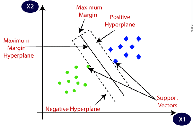
Support vector machine (SVM) is a supervised machine learning algorithm. Supervised machine learning algorithms train on labeled data i.e., data that has a matching output. SVM can be used for both classification and regression. It works by creating hyperplanes in a space that is multidimensional in order to create a separation of the different classes. The advantages of the support vector machine include Effectiveness in spaces that have high dimensions; If you have cases that the dimensions are higher than the sample number, SVM is still effective; They are efficient in terms of memory use because of their ability to use training points subsets. Some weaknesses of SVM are: They can lead to overfitting in cases where the feature number is greater than the sample size and they do not have a direct way of providing probability estimates.

Fig 1. Support vector machine diagram
2. Decision trees
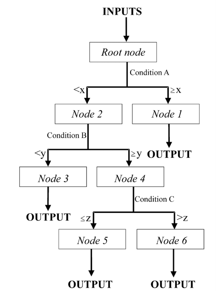
Decision trees (DT) are one of the simplest classification algorithms and can be used for both classification and regression. Depending on the turning of the parameters, decision trees can yield good results (Raj, 2021). DT derives its name from its structure which is tree like. DT are a set of rules that do the conversion of information such as image pixels to its appropriate class. The classification to classes is based on learning decision rules from the data features. Some of the advantages of DTs include; They are easy to interpret and understand because they can be visualized; less data preparation is required as compared to other algorithms; The DT can handle categorical and numerical data; because it is based on a white-box model, the results from a DT are easy to interpret; the reliability of the model can easily be tested using statistical methods. Even though it has its advantages, DT also has disadvantages such as; being prone to overfitting, it is, therefore, necessary to define the depth and the number of nodes for DT before training it; they are also not very stable, as different trees can be generated with slight variations in the data; they need prior balancing of the dataset before fitting to avoid the creation of biased trees.

Fig 1: Example of a decision tree, adapted from (Yang et al., 2003)
3. K-nearest neighbors
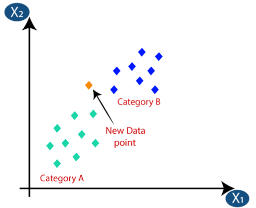
K-nearest neighbors(KNN) are regarded as one of the simplest classification algorithms for image classification. They work by identifying a number of training samples that are closest to the new point or thing to be classified and providing the classification based on those samples. For example, if you are trying to determine if an image is of a cat or dog using some dataset of cats and dogs, the KNN will create a grouping of the dataset and the new image will be classified according to the nearest distance to the clusters. If the image is near the dog cluster, it will be classified as a dog. The number of samples can be user-defined or determined by the density of the points. To use k-nearest neighbors for classification, you need to determine a metric such as the Euclidian distance that is commonly used. The choice of the metric to be used is dependent on the type of data one has. The success of K-nearest has been in cases of irregular decision boundaries. Some of the advantages of K-nearest neighbors include: Ease of interpretation, calculations performed faster and high levels of accuracy.

4. Artificial neural networks
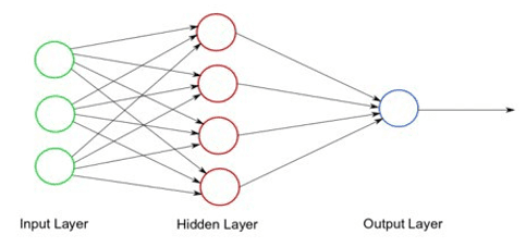
Artificial Neural Networks (ANN) are a result of trying to emulate the biological neural system. Their creation is done by programming computers to behave like interconnected cells in the brain. ANN is generally used to provide solutions to problems that have a noisy dataset and have no linear ties. The ANN model can be generated from the data available and can be adapted to problems from a wide range. ANN is not well fitted to solve problems that are well-defined and deterministic.

Fig 3: Artificial Neural networks
The Convolutional neural network (CNN) which is a special type of ANN has been used to improve the accuracy of image detection of ANN. CNN often contains one or two convolutional layers and then preceded and followed by input and output dense layers respectively. Convolutional layers work as a filter to bring to focus the dominant features of an image. By applying convolutional layers, the accuracy of an ANN in classifying an image improves. There are other variations of ANN that are used to improve performance based on the type of the data being classified such as Long Short-Term Memory (LSTM) and Recurrent Neural Network (RNN).
5. Naive Bayes classification
Naive Bayes are algorithms are based on methods for Bayesian classification which are derived from the Bayesian theory. Naive Bayes is a probability-based method. The label with the highest probability becomes the label for the given image that is being classified based on the selected features. In other words, given the features in an image, what is the probability of that image belonging to a certain label. Naive Bayes models are regarded to be fast and most suitable for high-dimensional data. The algorithms are named naïve based on the fact that you have to make naïve assumptions about the generative model that is used to generate the labels. The Gaussian naïve Bayes (GNV) makes the assumption that the Gaussian distribution is the source of data for each label. The GNV has the advantage of being easy to understand. Multinomial naïve Bayes makes the assumption that data is generated from multinomial distributions that are simple.
The advantages of naïve Bayes classification include; their ability to be easily interpreted, few tunable parameters, and that the provided probabilistic predictions are straightforward. Naïve Bayes classifications are mostly used as the starting point classifiers before you explore more complicated classifiers. They are most preferred when the complexity of the model is not of any importance.
REFERENCES
Parekh, R. (2021). Fundamentals of Image, Audio, and Video Processing Using Matlab.
Raj, A. (2021). An Exhaustive Guide to Decision Tree Classification How are Decisions Made in a Decision Tree ?
Yang, C. C., Prasher, S. O., Enright, P., Madramootoo, C., Burgess, M., Goel, P. K., & Callum, I. (2003). Application of decision tree technology for image classification using remote sensing data. Agricultural Systems, 76(3), 1101–1117. https://doi.org/10.1016/S0308-521X(02)00051-3
Zhau, S. K. (2016). Medical Image Recognition, Segmentation and Parsing. In Medical Image Recognition, Segmentation and Parsing. https://doi.org/10.1016/c2014-0-02794-3


