What is MNIST? And why is it important?

To follow this tutorial, you should have some prior basic knowledge of Machine Learning including Neural Networks, as well as basic programming knowledge in any language (preferably in Python). Other than that, the rest of the article is pretty beginner-friendly.

We will also be using Colaboratory offered by Google for writing our code.

Our task is to classify a given image of a handwritten digit into one of 10 classes representing integer values from 0 to 9, inclusively using a CNN that will be able to recognize the handwritten digits. CNN is a type of deep neural network commonly used for computer vision applications. So we will build an image classifier TensorFlow’s Keras API on the MNIST dataset. Keras is a Python library and is highly recommended for beginners due to its smooth learning curve. It is very commonly used in implementing neural networks. For more on Keras, follow this link.

Step 1: Importing and Exploring the MNIST Dataset

 

The example below loads the MNIST dataset using the Keras API. The digit images are separated into two groups: x_train, x_test and y_train, y_test. The x_train and x_test parts contain greyscale RGB codes (from 0 to 255). The y_train and y_test parts contain labels from 0 to 9.

 

# Loading mnist dataset
from keras.datasets import mnist
(x_train, y_train), (x_test, y_test) = mnist.load_data()

The digit images are separated into two sets: training and test. The x_train and x_test parts contain greyscale RGB codes (from 0 to 255). The y_train and y_test parts contain labels from 0 to 9. We can see that the training set contains 60,000 images while the test set contains 10,000 images and that the images are indeed square with 28×28 pixels by running the example below:

# Displaying dataset summary
print('X_train = %s, Y_train = %s' % (x_train.shape, y_train.shape))
print('X_test = %s, Y_test = %s' % (x_test.shape, y_test.shape))

 

Output:

 

X_train = (60000, 28, 28), Y_train = (60000)
X_test = (10000, 28, 28), Y_test = (10000)

 

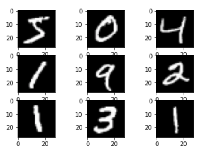
A plot of the first nine images in the dataset can also be seen by running the following code:

 

# Plot of first 9 images in mnist dataset
import matplotlib.pyplot as plt
for x in range(9):
    plt.subplot(330 + 1 + x)
    plt.imshow(x_train[x], cmap=plt.get_cmap('gray'))
plt.show()

 

Output:

 

![](https://res.cloudinary.com/carpool199/image/upload/v1584625154/img1.png)

Step 2: Reshaping the images in the dataset

 

We need to reshape the dataset to 4-dimensional NumPy arrays to be able to use it in Keras. From seeing one of the outputs above, we know that the dataset is 3-dimensional, since x_train represents (60000,28,28), where 60000 is the number of images in the train set and (28,28) represents the size of each image. So let’s convert these to 4-dimensional arrays using the following code:

 

# Reshaping the array to become 4-dimensional
x_train = x_train.reshape(x_train.shape[0], 28, 28, 1)
x_test = x_test.reshape(x_test.shape[0], 28, 28, 1)
input_shape = (28, 28, 1)
# To ensure decimal points after division
x_train = x_train.astype('float32')
x_test = x_test.astype('float32')
print('After reshaping, x_train is :', x_train.shape)
print('x_train contains', x_train.shape[0], "images")
print('x_test contains', x_test.shape[0], "images")

 

Output:

 

After reshaping, x_train is : (60000, 28, 28, 1)
x_train contains 60000 images
x_test contains 10000 images

Step 3: Normalizing the images in the dataset

 

Normalization is the process of changing the range of pixel intensity values to bring the image into a range that is more familiar or normal to the senses. We must normalize our data as it is always required in neural network models. This can be achieved by dividing the RGB codes by 255, which is the maximum RGB code minus the minimum RGB code (255 -0 ). So let’s normalize our images using the following code:

 

# Normalizing the images by dividing by the max RGB value (255)
x_train /= 255
x_test /= 255

Step 4: Constructing the Convolutional Neural Network

 

Models and Layers are the building blocks of Keras and they help you to construct the deep neural networks. So we will be creating a sequential model and will start adding layers to it. The model consists of two components:

1. Feature extraction front end consisting of convolutional and pooling layers
2. Classifier backend that will make a prediction

 

For the feature extraction front-end, we start with the 2D convolutional layer with 32 filters and a kernel size of (3,3). This layer is basically a mask and can be used for blurring, sharpening, embossing, and edge detection within an image. It uses the activation function Rectifier Linear Unit — ReLU. The activation function is the heart of a deep neural network and without it, you can only fit a linear model to your data. The convolutional layer is followed by a max-pooling layer. The filter maps can then be flattened to provide features to the classifier.

 

As this is a multiclass classification problem with 10 possible outcomes (there are 10 digits overall from 0 to 9), the output layer will consist of 10 nodes, requiring the softmax activation function which is best for multiclass classification tasks. We have also added a dense layer to interpret the features with 100 nodes. The code of the provided explanation of the model is as follows:

 

# Creating a  sequential model named and adding layers to it
from keras import models
from keras import layers
network = models.Sequential()
network.add(layers.Conv2D(32, (3, 3), activation='relu', kernel_initializer='he_uniform', input_shape=(28, 28, 1)))
network.add(layers.MaxPooling2D((2, 2)))
network.add(layers.Flatten())
network.add(layers.Dense(100, activation='relu', kernel_initializer='he_uniform'))
network.add(layers.Dense(10, activation='softmax'))

Step 5: Compiling and fitting the model

 

Till now, we have created an empty CNN which is not optimized. So, we will now compile our network by providing 3 key parameters: the optimizer, loss function, and the metrics that we will monitor.

 

There are different types of optimizers, loss functions, and metrics, however, we will not delve into the details of these. All you need to for this example is that we have chosen Adam as the optimization algorithm as it is efficient and best suited for problems with a lot of parameters, like our own. For the loss function, we have opted for Sparse Categorical Crossentropy as we are dealing with a multiclass classification problem. This function effectively computes the difference between the actual output and the output predicted by the model which in turn is the error in the prediction. This error is given as feedback to the optimizer (Adam) which comes up with a better model in each and every iteration. For our metric to be monitored, we have chosen accuracy which is pretty standard.

 

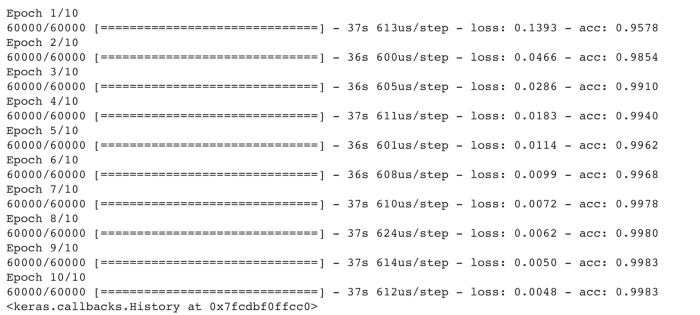
Lastly, we have used the fit method to train the model on the dataset and we have gone for 10 training epochs. Epoch is the number of times you iterate over the entire dataset. The code for this is as follows:

 

network.compile(optimizer='adam', 
              loss='sparse_categorical_crossentropy', 
              metrics=['accuracy'])
network.fit(x=x_train,y=y_train, epochs= 10)

 

Output:

 

Step 6: Performance Evaluation

 

As the final step, we have evaluated the trained model with x_test and y_test using just one line of code:

 

# Determining the accuracy of the trained model
network.evaluate(x_test, y_test)

 

Output:

 

 

As can be seen above, we have achieved an accuracy of 98.78% which is pretty good.